

Modeling COVID-19 spread and control
- Mathias Talmant

- 26 mars 2020
- 10 min de lecture
COVID-19 Series

ABSTRACT
One of the most prominent frameworks used by epidemiologists to model the spread of a disease is known as SIR, which stands for Susceptibles, Infected and Removed (Kermack & McKendrick, 1927). Given a set of assumptions detailed hereafter, a static picture of the current outbreak (24/03/2020) led me to the following conclusions:
If all parameters were kept constant for a year, the infection peak would be reached on July 15, 2020 and less than 1% of the world population would be spared by COVID-19 after one year. Assuming a 3% Case Fatality Rate, the total cumulative number of deaths would amount to 231,266,604 deaths on 24/03/2021. The main reason for such serious prediction is that the infected cases rise exponentially, but the recovered population rises only linearly. Please consider this estimate as a maximum because it assumes the current state will persist for one year with no improvement or deterioration.
I obtained a basic reproduction rate of 7, which means that 1 individual with COVID-19 will typically infect 7 other individuals. This is more than twice as much as SARS coronavirus, but with a fourth of its Case Fatality Rate. Therefore, it seems that COVID-19’s main threat is its scale, not its lethality.
Herd immunity would be reached by vaccinating 86% of the world population, but it is almost impossible to reach considering the time needed to develop a vaccine and the scalability limit of the manufacturing and distribution processes. Vaccination is a long-term solution to the problem, but in the short-term, we need to respect quarantines, increase hospitals’ capacity, protect health professionals and multiply trials to find a cure.
I. METHODOLOGY
II. VARIABLES
III. FORMULAS
IV. ASSUMPTIONS
V. RESULTS AND INTERPRETATIONS
VI. LIMITS
VII. APPENDIX
I. METHODOLOGY
Mathematical models are ubiquitous in the study of the transmission dynamics of infectious diseases. They are valuable to governments because they show the likely outcome of an epidemic and help evaluating potential control strategies for public health interventions. Several approaches can be used to uncover the mechanisms behind the spread of a disease, but in this article I will be focusing on the SIR model (Kermack & McKendrick, 1927), a system of communicating vessels. The population consists of only three types of individuals (Susceptible, Infected and Removed), whose number are functions of time, a rate of infection and a recovery rate. When a new infection occurs, the infected individual moves from the Susceptible class to the Infected class. Infected individuals, ie. reported cases and silent spreaders, are capable of spreading the disease to the susceptible category only. Those individuals who have been infected can only move to the Removed category, after a certain period of time, either due to immunization, isolation or death.
SUSCEPTIBLE – S(t) represents the number of individuals not yet infected with the disease at time t.
INFECTED – I(t) denotes the number of infected individuals at time t.
REMOVED – R(t) refers to the number of individuals that can no longer contract the disease at time t.

II. VARIABLES
β is the transmission coefficient or rate of infection (from S to I).
γ is the recovery coefficient (from I to R).
R0 is the basic reproduction number, ie. the expected number of cases directly generated by an infected individual in a population of susceptible individuals.
ρ is the proportion of people that need to be vaccinated to achieve herd immunity and put an end to the disease outbreak, computer as 1-1/ R0.
CFR is the Case Fatality Rate, ie. proportion of infected individuals that result in deaths.
λ is the adjustment coefficient applied to the number of reported cases to account for non-diagnosed COVID-19 infections.
N is the world population in 2020, according to the United Nations.
III. FORMULAS

S’, I’ and R’ are respectively the rates of change for S, I and R.

S(0) = N
I(0) = Reported Cases0*(1+λ)
R(0) = Removed0
S(1) = S(0) + S’(0)
I(1) = I(0) + I’(0)
R(1) = R(0) + R’(0)
IV. ASSUMPTIONS
To make the model as general as possible and in order to simplify computations, I had to consider the following set of assumptions :
All individuals in the world population are equally susceptible to contract the disease at time t = 0 and their age and gender distribution is uniformly distributed.
The rate of infection and recovery is much faster than the time scale of births and deaths and therefore, these factors are ignored.
The average transmissibility among individuals ignores individual variations.
It has not been proven yet, but I will assume that people who recovered from COVID-19 are not able to be infected again or to transmit the infection to others.
Individuals are infectious immediately, although in reality there typically is a lag.
Knowing that “86% of all infections were undocumented (95% CI: [82%–90%]) prior to 23 January 2020 travel restrictions” in China, it seems reasonable to multiple the number of reported cases by two to account for non-recorded silent spreaders. The latter ones are individuals who are infectious but show no symptoms and thus have not been tested yet.
There is a significant discrepancy in case mortality rate across regions and age, but I will assume a constant average rate of 3%, based on observations in the Hubei province in China. This is a conservative estimate because in 2003, while the 2003 SARS epidemic was still ongoing, the WHO reported a fatality rate of as low as 3%, whereas the final case fatality rate ended up being 9.6%.
Hospitals’ capacity was ignored while estimating the mortality rate as it can differ widely according to countries.
V. RESULTS AND INTERPRETATIONS
My base case scenario was estimated on March 24/03/2020. β and γ were estimated as the average of the last seven observations of S, I and R (from 17/03/2020 to 24/03/2020). Please refer to the end of the document for data sources.


The SIR model is very sensitive to change in the value of β and γ. These parameters can be very volatile, hence why it is difficult to give a static picture of an epidemic forecast.
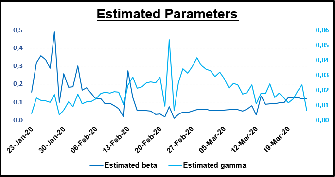
Not surprisingly, since β and γ can vary from one day to another, this graph shows how volatile the basic reproduction can be. On March 24, 2020 it was 4.38, which means that on average one infected individual with COVID-19 will typically infect 4.38 susceptible individuals.

The graph of the base case scenario is typical of an epidemic. As the virus is spreading, the number of infected individuals grows faster and faster before it reaches a ceiling. In parallel, the number of sound individuals decline faster until everyone is either infected or removed (immunised or dead). Governments’ objective is to flatten the curve and fall below the maximum capacity level of hospitals. This level is not represented here, because it is very hard to estimate an average given world discrepancy. However, it is certain that this critical level will be exceeded soon as we approached the infection peak. This is even more likely if governments cannot guarantee the safety of their health care professionals, who are the most critical to flatten the curve, but also the most at risk of falling sick.

Linear scale (on the left) applies to Susceptible, Infected and Removed.
Log scale (on the right) applies to Death.
The point at which the daily number of new removed cases should exceed the daily number of new infected cases, or improvement threshold, is expected to be in mid-August. This assumes that we keep the parameters constant up to this point. In other words, the quarantine could possibly continue for several more months until the end of the summer 2020.

Log scale (on the right applies to Infected, Death and Removed.
Here, λ is used as an adjustment factor to β and γ for the purpose of the scenario analysis. For example, when λ = -10%, I deteriorated R0 of the base case scenario by increasing β and decreasing γ by 10%.

If all parameters were kept constant for a year, given the base case scenario, the infection peak would be reached on July 15, 2020 and less than 1% of the world population would be spared by COVID-19, leading to a total cumulative number of deaths of 231,266,604 deaths. Herd immunity would be reached by vaccinating 86% of the world population. This is almost impossible to reach, especially over a year.
If both the infection rate and the recovery rate worsened by 50%, the infection peak would be reached on June 8, 2020 and 8% of the world population would be spared by COVID-19, leading to a total cumulative number of deaths of 216,411,236 deaths after one year. In this case, the epidemic would be completely out of control with a basic reproduction rate of 21. I think the lower number of deaths compared to the base case scenario, despite worsening parameters, is due to faster rate of infection leading to more deaths more quickly. This is even more true if we consider that when the number of critical cases requiring hospitalisation exceeds the capacity, some patients can’t be taken care of and mortality thus increases. As sad as it is, when individuals die, they can no longer spread the disease, which can help to slow down the epidemic. Herd immunity would be reached by vaccinating 95% of the world population. This level is very unlikely to be reached any time soon.
If both the infection rate and the recovery rate improved by 50%, the infection peak would be reached on December 29, 2020 and 28% of the world population would be spared by COVID-19, leading to a total cumulative number of deaths of 167,849,366 deaths after one year. At this stage, the epidemic would almost be under control with a basic reproduction rate of 2, but further efforts would be needed to lower it below the critical threshold of 1. The lower number of deaths compared to the base case scenario can easily be explained by measures taken by the government to limit social interactions and travels along with new therapeutics. Herd immunity would be reached by vaccinating 57% of the world population. This is a more realistic target, yet it will still take years to achieve and in the meantime, COVID-19 may evolve and require a different vaccine.
In my opinion, the difficulty to reach herd immunity entails the non-significance of a vaccine in the short-term. It is very unlikely that we can find a vaccine soon enough and scale up the production on a global scale in order to reach the critical ρ. My rough estimate of the number of vaccines we could get by the end of the year assuming that we start production in mid-June to mid-July would be around 150,000,000, which is negligible in the short-term. Besides, the critical ρ value assumes a vaccine efficacy of 100%, but studies show that it may be far less for some vaccines. This is why I did not try to model a scenario with vaccination.
Vaccination is a long-term solution to the problem, but in the short-term, we need to respect quarantines, increase hospitals’ capacity and multiply trials to find a cure. In the coming weeks, I will release another article dealing with the treatments being tested to eradicate COVID-19.
R0 is closely monitored by governments because it shows how much an epidemic is spreading. When R0 > 1, ΔI > ΔR, which means that more individuals join the Infected class than the Removed class. This is what everyone wants to avoid. When R0 < 1, ΔI < ΔR, which means that more individuals join the Infected class than the Removed class. This is what we want. Knowing that the number of cases reported every day is still skyrocketing in late March 2020, it is very likely that the infection peak is well ahead of us. As evidenced by the sensitivity analysis, lots of efforts will be needed to reach the top left corner where the basic reproduction rate nears the critical value of 1.

10% increment
In my base case scenario, I obtained a basic reproduction rate of 7, which means that the epidemic is spreading a lot faster than MERS or SARS coronavirus. However, the CFR is a lot lower, especially if we compare it to the Ebola epidemic. Thus, we can conclude that given the information we have now, COVID-19’s main threat seems to be its scale, but not its lethality.

Source: Dr Melvin Sanicas, vaccinologist, on Twitter, 31/01/2020.
Let’s talk about business now. Indubitably, the outbreak of COVID-19 has knocked to the ground most equity indices along with oil, as shown in the graph. In early January 2020, France, Europe, the US and China followed the same trend initially, although China was relatively lower since it was the first casualty of virus. In early March, the fall continued China succeeded to limit the damage while Eastern economies are now feeling the consequences of their late actions. In late March, there seems to be some recovery in some share prices, but it may be a bull trap before another collapse as we are only at the beginning of the outbreak in my opinion. Crude oil was the first to decline due to a price war between Saudi Arabia and Russia on output cuts, but the sharp decrease in price intensified as the epidemic unfolded. Gold seems to be the only safe haven in times of market turmoil. An analysis of the economic consequences, the government responses and my takes on some investment classes will come in other articles in the coming weeks.

Sources: Yahoo Finance, Johns Hopkins University & Medecine.
Europe – STOXX 600 (^STOXX)
France – CAC40 (^FCHI)
United States – S&P500 (^GSPC)
China – Hang Seng (^HSI)
Gold – Gold Future (GC=F)
Oil - Crude Oil (CL=F)
VI. LIMITS
Models are only as good as the assumptions on which they are based. I do not have the pretention to say that my predictions will come true. It is a best guess estimate given my assumptions, the data I could find online and my personal statistical knowledge. One of the biggest assumptions I had to use for the SIR model is that individuals either die or become immune after they have been infected. This statement has not been confirmed by the WHO. In addition, the rate at which the disease is spreading is volatile, data can be incomplete and future discovery of a vaccine can have a significant impact on my forecasts. My estimates of β and γ were based on an average of the last seven days, as of March 24, 2020. This entails that my forecasts are valid if these parameters do not change in the course of the year. However, this is not realistic because parameters are non-static, they change every day as the epidemic evolves. Measures taken by government, intensive research on therapeutics and Therefore this analysis should
VII. APPENDIX
Academic Paper
Kermack, W. O. and McKendrick, A. G. (1927). "A Contribution to the Mathematical Theory of Epidemics".
Data
Relevant links
The above references an opinion and is for information purposes only. It is not intended to be investment advice. Seek a duly licensed professional for investment advice.
MT Finance - Mathias Talmant.


Commentaires